A simple symbolic regression example
This notebook implements a symbolic regression pipeline based on Genetic Programming (GP) using the flex framework and its custom GPSymbolicRegressor.
The goal is to discover analytical expressions that best fit a given PMLB dataset by:
evolving symbolic expressions;
optimizing embedded numerical constants;
penalizing overly complex expressions;
evaluating performance on training and test datasets.
The code supports:
multi-variable regression problems;
automatic constant tuning using gradient-based optimization;
parallel execution using Ray.
Imports and Dependencies
First, we import all the required libraries for:
Genetic Programming:
deap.gp, customflex.gputilitiesNumerical computation:
numpy,mygradOptimization:
pygmo(for constant fitting)Machine Learning utilities:
scikit-learnParallelism:
rayDataset generation: custom
generate_datasetfunction
The code relies on both evolutionary optimization (for structure) and gradient-based optimization (for constants).
[1]:
%env RAY_ACCEL_ENV_VAR_OVERRIDE_ON_ZERO=0
env: RAY_ACCEL_ENV_VAR_OVERRIDE_ON_ZERO=0
[2]:
from deap import gp

from flex.gp import regressor as gps
from flex.gp.util import (
    detect_nested_trigonometric_functions,
    load_config_data,
    compile_individual_with_consts,
)
from flex.gp.primitives import add_primitives_to_pset_from_dict
import numpy as np
import ray

import warnings
import pygmo as pg

import re
from sklearn.metrics import r2_score

import time

import mygrad as mg
from mygrad._utils.lock_management import mem_guard_off

from functools import partial


from sklearn.model_selection import train_test_split
from sklearn.preprocessing import StandardScaler
from pmlb import fetch_data

import matplotlib.pyplot as plt
[3]:
# set up number of cpus per ray worker
num_cpus = 1
[4]:
# --- Custom generate dataset function ---
def generate_dataset(problem: str="1027_ESL", random_state: int=42, scaleXy: bool=True):
    np.random.seed(42)
    num_variables = 1
    scaler_X = None
    scaler_y = None

    # PMLB datasets
    X, y = fetch_data(problem, return_X_y=True, local_cache_dir="./datasets")

    num_variables = X.shape[1]

    X_train, X_test, y_train, y_test = train_test_split(
        X, y, test_size=0.25, random_state=random_state
    )

    y_train = y_train.reshape(-1, 1)
    y_test = y_test.reshape(-1, 1)

    if scaleXy:
        scaler_X = StandardScaler()
        scaler_y = StandardScaler()

        X_train_scaled = scaler_X.fit_transform(X_train)
        y_train_scaled = scaler_y.fit_transform(y_train)
        X_test_scaled = scaler_X.transform(X_test)
    else:
        X_train_scaled = X_train
        y_train_scaled = y_train
        X_test_scaled = X_test

    y_test = y_test.flatten()
    y_train_scaled = y_train_scaled.flatten()

    num_train_points = X_train.shape[0]


    # note y_test and y_train_scaled must be flattened
    return (
        X_train_scaled,
        y_train_scaled,
        X_test_scaled,
        y_test,
        scaler_X,
        scaler_y,
        num_variables,
        num_train_points,
    )
Evaluation Function and Constant Optimization
The core of the symbolic regression pipeline is the definition of the fitness function. First, we need to define an error measure, which in this case will be the standard MSE between the targets and the predictions. However, we remark that each individual carries some numerical constants that need to be optimized as well. For example, the individual
may have a near 0 fitness for a given triple \((c_1, c_2, c_3)\) and a very large fitness for other triples. This simple examples shows that it is important to auto-optimize carefully the constants in each individual.
If the evaluation function is differentiable, then one natural choice to auto-optimize constants is the use of any gradient-based solver. In this example, we are going to use the library mygrad for autodifferentiation and pygmo for the optimization routine.
[5]:
def eval_model(individual, X, consts=[]):
    num_variables = X.shape[1]
    if num_variables > 1:
        X = [X[:, i] for i in range(num_variables)]
    else:
        X = [X]
    warnings.filterwarnings("ignore")
    y_pred = individual(*X, consts)
    return y_pred


def compute_MSE(individual, X, y, consts=[]):
    y_pred = eval_model(individual, X, consts)
    MSE = np.mean((y - y_pred) ** 2)

    if np.isnan(MSE) or np.isinf(MSE):
        MSE = 1e8

    return MSE


def eval_MSE_and_tune_constants(tree, toolbox, X, y):
    individual, num_consts = compile_individual_with_consts(tree, toolbox)

    if num_consts > 0:

        eval_MSE = partial(compute_MSE, individual=individual, X=X, y=y)

        x0 = np.ones(num_consts)

        class fitting_problem:
            def fitness(self, x):
                total_err = eval_MSE(consts=x)
                # return [total_err + 0.*(np.linalg.norm(x, 2))**2]
                return [total_err]

            def gradient(self, x):
                with mem_guard_off:
                    xt = mg.tensor(x, copy=False)
                    f =  mg.tensor(self.fitness(xt)[0], copy=False)
                    f.backward()
                return xt.grad

            def get_bounds(self):
                return (-5.0 * np.ones(num_consts), 5.0 * np.ones(num_consts))

        # PYGMO SOLVER
        prb = pg.problem(fitting_problem())
        algo = pg.algorithm(pg.nlopt(solver="lbfgs"))
        # algo = pg.algorithm(pg.pso(gen=10))
        # pop = pg.population(prb, size=70)
        algo.extract(pg.nlopt).maxeval = 10
        pop = pg.population(prb, size=1)
        pop.push_back(x0)
        pop = algo.evolve(pop)
        MSE = pop.champion_f[0]
        consts = pop.champion_x

        if np.isinf(MSE) or np.isnan(MSE):
            MSE = 1e8
    else:
        MSE = compute_MSE(individual, X, y)
        consts = []
    return MSE, consts
Expression Complexity and Structure Checks
These helper functions analyze individuals to:
count trigonometric functions;
detect nested trigonometric expressions;
penalize overly complex or pathological solutions.
They are later used to regularize the fitness function.
[6]:
def check_trig_fn(ind):
    return len(re.findall("cos", str(ind))) + len(re.findall("sin", str(ind)))


def check_nested_trig_fn(ind):
    return detect_nested_trigonometric_functions(str(ind))

def get_features_batch(
    individuals_batch,
    individ_feature_extractors=[len, check_nested_trig_fn, check_trig_fn],
):
    features_batch = [
        [fe(i) for i in individuals_batch] for fe in individ_feature_extractors
    ]

    individ_length = features_batch[0]
    nested_trigs = features_batch[1]
    num_trigs = features_batch[2]
    return individ_length, nested_trigs, num_trigs
Fitness and Prediction Functions
The fitness function combines:
prediction error (MSE),
structural penalties (expression length),
functional penalties (nested trigonometric functions).
A Tarpeian selection strategy is applied to discard very large trees early.
[7]:
def predict(individuals_batch, toolbox, X, penalty, fitness_scale):

    predictions = [None] * len(individuals_batch)

    for i, tree in enumerate(individuals_batch):
        callable, _ = compile_individual_with_consts(tree, toolbox)
        predictions[i] = eval_model(callable, X, consts=tree.consts)

    return predictions


def compute_MSEs(individuals_batch, toolbox, X, y, penalty, fitness_scale):

    total_errs = [None] * len(individuals_batch)

    for i, tree in enumerate(individuals_batch):
        callable, _ = compile_individual_with_consts(tree, toolbox)
        total_errs[i] = compute_MSE(callable, X, y, consts=tree.consts)

    return total_errs


def compute_attributes(individuals_batch, toolbox, X, y, penalty, fitness_scale):

    attributes = [None] * len(individuals_batch)

    individ_length, nested_trigs, num_trigs = get_features_batch(individuals_batch)

    for i, tree in enumerate(individuals_batch):

        # Tarpeian selection
        if individ_length[i] >= 50:
            consts = None
            fitness = (1e8,)
        else:
            MSE, consts = eval_MSE_and_tune_constants(tree, toolbox, X, y)
            fitness = (
                fitness_scale
                * (
                    MSE
                    + 100000 * nested_trigs[i]
                    + 0.0 * num_trigs[i]
                    + penalty["reg_param"] * individ_length[i]
                ),
            )
        attributes[i] = {"consts": consts, "fitness": fitness}
    return attributes


def assign_attributes(individuals_batch, attributes):
    for ind, attr in zip(individuals_batch, attributes):
        ind.consts = attr["consts"]
        ind.fitness.values = attr["fitness"]
Main Training and Evaluation Pipeline
The following cell orchestrates the entire symbolic regression process:
loads configuration from a YAML file;
generates training and test datasets;
builds the GP primitive set;
initializes the symbolic regressor;
trains the model;
evaluates performance on training and test sets.
[8]:
regressor_params, config_file_data = load_config_data("simple_sr.yaml")

scaleXy = config_file_data["gp"]["scaleXy"]

# generate training and test datasets
(
    X_train_scaled,
    y_train_scaled,
    X_test_scaled,
    y_test,
    _,
    scaler_y,
    num_variables,
    _,
) = generate_dataset("1096_FacultySalaries", scaleXy=scaleXy, random_state=29802)

if num_variables == 1:
    pset = gp.PrimitiveSetTyped("Main", [float], float)
    pset.renameArguments(ARG0="x")
elif num_variables == 2:
    pset = gp.PrimitiveSetTyped("Main", [float, float], float)
    pset.renameArguments(ARG0="x")
    pset.renameArguments(ARG1="y")
else:
    pset = gp.PrimitiveSetTyped("Main", [float] * num_variables, float)

pset = add_primitives_to_pset_from_dict(pset, config_file_data["gp"]["primitives"])

batch_size = config_file_data["gp"]["batch_size"]
if config_file_data["gp"]["use_constants"]:
    pset.addTerminal(object, float, "c")

callback_func = assign_attributes
fitness_scale = 1.0

penalty = config_file_data["gp"]["penalty"]
common_params = {"penalty": penalty, "fitness_scale": fitness_scale}

gpsr = gps.GPSymbolicRegressor(
    pset_config=pset,
    fitness=compute_attributes,
    predict_func=predict,
    score_func=compute_MSEs,
    common_data=common_params,
    callback_func=callback_func,
    print_log=True,
    num_best_inds_str=1,
    save_best_individual=False,
    output_path="./",
    seed_str=None,
    batch_size=batch_size,
    num_cpus=num_cpus,
    remove_init_duplicates=True,
    **regressor_params,
)

tic = time.time()
gpsr.fit(X_train_scaled, y_train_scaled)
toc = time.time()

best = gpsr.get_best_individuals(n_ind=1)[0]

if hasattr(best, "consts"):
    print("Best parameters = ", best.consts)

print("Elapsed time = ", toc - tic)
individuals_per_sec = (
    (gpsr.get_last_gen() + 1)
    * gpsr.num_individuals
    * gpsr.num_islands
    / (toc - tic)
)
print("Individuals per sec = ", individuals_per_sec)

u_best = gpsr.predict(X_test_scaled)

# de-scale outputs before computing errors
if scaleXy:
    u_best = scaler_y.inverse_transform(u_best.reshape(-1, 1)).flatten()

MSE = np.mean((u_best - y_test) ** 2)
r2_test = r2_score(y_test, u_best)
print("MSE on the test set = ", MSE)
print("R^2 on the test set = ", r2_test)

pred_train = gpsr.predict(X_train_scaled)

if scaleXy:
    pred_train = scaler_y.inverse_transform(pred_train.reshape(-1, 1)).flatten()
    y_train_scaled = scaler_y.inverse_transform(
        y_train_scaled.reshape(-1, 1)
    ).flatten()

MSE = np.mean((pred_train - y_train_scaled) ** 2)
r2_train = r2_score(y_train_scaled, pred_train)
print("MSE on the training set = ", MSE)
print("R^2 on the training set = ", r2_train)

# ray is explicitly shut down at the end of the execution to release computational resources
ray.shutdown()
2026-02-25 11:18:31,563 INFO worker.py:1998 -- Started a local Ray instance. View the dashboard at http://127.0.0.1:8265
Generating initial population(s)...
 Removing duplicates from initial population(s)...
 DONE.
DONE.
Evaluating initial population(s)...
DONE.
 -= START OF EVOLUTION =-
                           fitness                           size
                ------------------------------  ------------------------------
gen     evals   min     avg     max     std     min     avg     max     std
1       2000    0.1103  0.6129  1.1296  0.3316  2       8.0595  21      3.8143
Best individuals of this generation:
sub(mul(c, ARG1), mul(c, add(ARG2, ARG1)))
2       2000    0.1103  0.3508  0.7454  0.1588  2       8.302   24      4.1524
Best individuals of this generation:
sub(mul(c, ARG1), mul(c, add(ARG2, ARG1)))
3       2000    0.1103  0.247   0.3748  0.075   2       7.982   24      4.2672
Best individuals of this generation:
sub(mul(c, ARG1), mul(c, sub(ARG2, ARG1)))
4       2000    0.1061  0.2048  0.2911  0.0589  2       8.306   26      4.397
Best individuals of this generation:
aq(ARG1, mul(sub(ARG2, ARG1), sub(add(ARG2, ARG3), c)))
5       2000    0.1061  0.1666  0.2527  0.0349  3       9.182   30      4.6258
Best individuals of this generation:
aq(ARG1, mul(sub(ARG2, ARG1), sub(add(ARG2, ARG3), c)))
6       2000    0.1061  0.1456  0.1732  0.0135  3       8.649   25      4.5359
Best individuals of this generation:
aq(ARG1, mul(sub(ARG2, ARG1), sub(add(ARG2, ARG3), c)))
7       2000    0.1061  0.1388  0.1532  0.0085  3       8.7245  25      4.6155
Best individuals of this generation:
aq(ARG1, mul(sub(ARG2, ARG1), sub(add(ARG2, ARG3), c)))
8       2000    0.1025  0.135   0.1453  0.0064  3       8.984   26      4.6724
Best individuals of this generation:
aq(sub(mul(c, ARG1), sin(ARG2)), sub(mul(c, ARG2), mul(c, ARG1)))
9       2000    0.1025  0.1326  0.14    0.0052  3       8.775   26      4.217
Best individuals of this generation:
aq(sub(mul(c, ARG1), sin(ARG2)), sub(mul(c, ARG2), mul(c, ARG1)))
10      2000    0.1025  0.1309  0.1368  0.0046  3       7.96    26      4.1211
Best individuals of this generation:
aq(sub(mul(c, ARG1), sin(ARG2)), sub(mul(c, ARG2), mul(c, ARG1)))
11      2000    0.1025  0.1296  0.135   0.0044  3       7.452   26      4.1453
Best individuals of this generation:
aq(sub(mul(c, ARG1), sin(ARG2)), sub(mul(c, ARG2), mul(c, ARG1)))
12      2000    0.1025  0.1287  0.1332  0.0043  3       6.97    25      4.1004
Best individuals of this generation:
aq(sub(mul(c, ARG1), sin(ARG2)), sub(mul(c, ARG2), mul(c, ARG1)))
13      2000    0.1025  0.1277  0.1321  0.0043  3       6.9555  28      4.2998
Best individuals of this generation:
aq(sub(mul(c, ARG1), sin(ARG2)), sub(mul(c, ARG2), mul(c, ARG1)))
14      2000    0.1025  0.127   0.1311  0.0044  3       7.129   28      4.4758
Best individuals of this generation:
aq(sub(mul(c, ARG1), sin(ARG2)), sub(mul(c, ARG2), mul(c, ARG1)))
15      2000    0.1025  0.1262  0.131   0.0044  3       7.443   28      4.7715
Best individuals of this generation:
aq(sub(mul(c, ARG1), sin(ARG2)), sub(mul(c, ARG2), mul(c, ARG1)))
16      2000    0.1025  0.1254  0.13    0.0045  3       7.3915  28      4.9913
Best individuals of this generation:
aq(sub(mul(c, ARG1), sin(ARG2)), sub(mul(c, ARG2), mul(c, ARG1)))
17      2000    0.1025  0.1247  0.129   0.0046  3       7.422   29      5.281
Best individuals of this generation:
aq(sub(mul(c, ARG1), sin(ARG2)), sub(mul(c, ARG2), mul(c, ARG1)))
18      2000    0.1025  0.1238  0.1284  0.0047  3       8.152   29      5.586
Best individuals of this generation:
aq(sub(mul(c, ARG1), sin(ARG2)), sub(mul(c, ARG2), mul(c, ARG1)))
19      2000    0.1025  0.123   0.1274  0.0049  3       8.9855  29      5.7858
Best individuals of this generation:
aq(sub(mul(c, ARG1), sin(ARG2)), sub(mul(c, ARG2), mul(c, ARG1)))
20      2000    0.1025  0.1222  0.127   0.0049  3       10.028  29      5.8074
Best individuals of this generation:
aq(sub(mul(c, ARG1), sin(ARG2)), sub(mul(c, ARG2), mul(c, ARG1)))
 -= END OF EVOLUTION =-
The best individual is aq(sub(mul(c, ARG1), sin(ARG2)), sub(mul(c, ARG2), mul(c, ARG1)))
The best fitness on the training set is 0.1025
Best parameters =  [1.9244978  2.9227811  2.16785583]
Elapsed time =  89.945805311203
Individuals per sec =  466.9478454796689
MSE on the test set =  1.535581223536389
R^2 on the test set =  0.796316488032204
MSE on the training set =  2.2604829120253043
R^2 on the training set =  0.9115115245302139
[9]:
# get the sympy version of the best individual
best_expression_sympy_str = str(gpsr.get_best_individual_sympy())
best_expression_sympy_str
[9]:
'(1.9244978027630006*ARG1 - sin(ARG2))/sqrt((-2.1678558285490226*ARG1 + 2.922781097169807*ARG2)**2 + 1)'
Plots
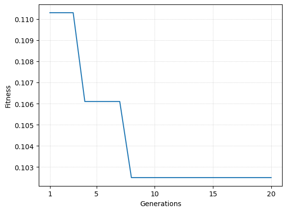
[10]:
fitness = gpsr.get_train_fit_history()
generations = gpsr.generations
plt.plot(np.arange(1, generations+1), fitness)
plt.xlabel("Generations")
plt.ylabel("Fitness")
plt.xticks([1, 5, 10, 15, 20])
plt.grid(True, linestyle=":", linewidth=0.5)
plt.show()
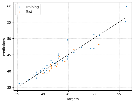
[11]:
y_min = min(np.min(y_train_scaled), np.min(y_test))
y_max = max(np.max(y_train_scaled), np.max(y_test))

plt.scatter(y_train_scaled, pred_train, s=5, label="Training")
plt.scatter(y_test, u_best, s=5, label="Test")
plt.plot([y_min, y_max], [y_min, y_max], "k--", linewidth=1)
plt.grid(True, linestyle=":", linewidth=0.5)
plt.xlabel("Targets")
plt.ylabel("Predictions")
plt.legend()
plt.show()